File:Symmetricwave2.png
原本檔案 (1,811 × 1,356 像素,檔案大細:540 KB ,MIME類型:image/png)

|
This physics image could be recreated using vector graphics as an SVG file. This has several advantages; see Commons:Media for cleanup for more information. If an SVG form of this image is already available, please upload it. After uploading an SVG, replace this template with {{vector version available|new image name.svg}}.
|
摘要
| 描述 |
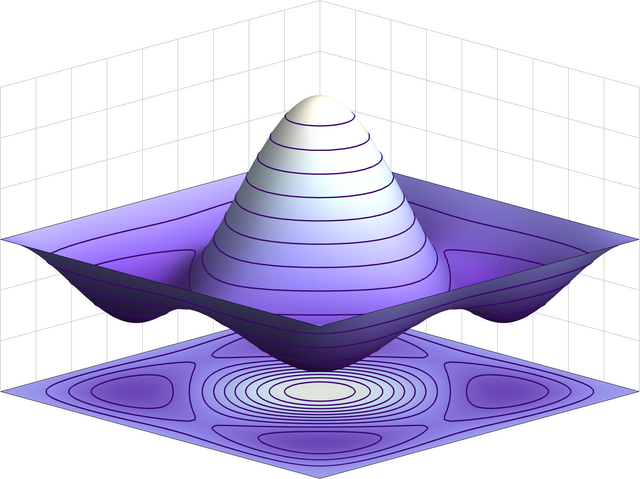
English: Symmetric wavefunction for a (bosonic) 2-particle state in an infinite square well potential. |
| 來源 | 自己作品 |
| 作者 | TimothyRias |
協議
我,呢份作品嘅作者,決定用以下許可發佈呢件作品:
Ĉi tiu dosiero estas disponebla laŭ la permesilo Krea Komunaĵo Atribuite 3.0 Neadaptita.
- 你可以:
- 去分享 – 複製、發佈同傳播呢個作品
- 再改 – 創作演繹作品
- 要遵照下面嘅條件:
- 署名 – 你一定要畀合適嘅表彰、畀返指向呢個授權條款嘅連結,同埋寫明有無改過嚟。你可以用任何合理方式去做,但唔可以用任何方式暗示授權人認可咗你或者你嘅使用方式。
摘要
This 3D graph shows the wavefunction for the 2-particle bosonic state for the one dimensional infinite square well at the same energy as the fermionic 2-particle groundstate. (See for example D.J. Griffiths, Introduction to quantum mechanics, Prentice Hall , 1995, section 5.1.1) The picture was created using Mathematica 6.0 using the following code:
$Assumptions = {n \[Element] Integers, m \[Element] Integers};
f[n_, x_] := Sqrt[2] Sin[n \[Pi] x];
s[n_, m_] :=
 Function[{x, y}, (f[n, x] f[m, y] + f[n, y] f[m, x])/Sqrt[2]];
swave2 = Plot3D[Evaluate[-s[3, 1][x, y]], {x, 0, 1}, {y, 0, 1},
  PlotPoints -> 35,
  PlotRange -> {-2.5, 3.5},
  MeshFunctions -> {#3 &},
  MeshStyle ->
   Directive[ColorData["DeepSeaColors"][.1], Thickness[.002]],
  Mesh -> 10,
  ColorFunction -> "LakeColors",
  BoxRatios -> {1, 1, .7},
  Boxed -> False,
  Axes -> False];
sgroundplot = Plot3D[-3, {x, 0, 1}, {y, 0, 1},
  MeshFunctions -> {s[1, 3][#1, #2] &},
  Mesh -> 10,
  MeshStyle ->
   Directive[ColorData["DeepSeaColors"][.1], Thickness[.002]],
  PlotPoints -> 50,
  ColorFunction -> (ColorData["LakeColors"][(-s[1, 3][#1, #2] + 2.5)/
      6] &)];
swave3 = Show[{swave2, sgroundplot},
 PlotRange -> {{0, 1}, {0, 1}, {-3, 3}},
 Axes -> None,
 PlotRangePadding -> None,
 ImagePadding -> 1,
 FaceGrids -> {
   {{-1, 0, 0}, {Table[i, {i, 0, 1, 1/9}],
     Table[i, {i, -3, 3, 1}]}},
   {{0, -1, 0}, {Table[i, {i, 0, 1, 1/9}], Table[i, {i, -3, 3, 1}]}}
   },
 ViewPoint -> 1000 {5, 5, 2},
 ViewVertical -> {0, 0, 1},
 ViewCenter -> {.5, .5, 0},
 ImageSize -> 600]
Export["Symmetricwave2.png", swave3, "PNG"]
檔案歷史
撳個日期/時間去睇響嗰個時間出現過嘅檔案。
| 日期/時間 | 縮圖 | 尺寸 | 用戶 | 註解 | |
|---|---|---|---|---|---|
| 現時 | 2024年2月19號 (一) 15:52 |  | 1,811 × 1,356(540 KB) | Jähmefyysikko | Antialiasing and higher resolution |
| 2008年10月15號 (三) 13:18 |  | 600 × 450(79 KB) | TimothyRias | {{Information |Description= |Source= |Date= |Author= |Permission= |other_versions= }} Category:Physics plots | |
| 2008年10月7號 (二) 14:52 |  | 360 × 286(25 KB) | TimothyRias | {{Information |Description={{en|1=Symmetric wavefunction}} |Source=Own work by uploader |Author=TimothyRias |Date= |Permission= |other_versions= }} <!--{{ImageUpload|full}}--> |
檔案用途
以下嘅1版用到呢個檔:
全域檔案使用情況
下面嘅維基都用緊呢個檔案:
- ar.wikipedia.org嘅使用情況
- ast.wikipedia.org嘅使用情況
- ca.wikipedia.org嘅使用情況
- da.wikipedia.org嘅使用情況
- en.wikipedia.org嘅使用情況
- eu.wikipedia.org嘅使用情況
- fa.wikipedia.org嘅使用情況
- ga.wikipedia.org嘅使用情況
- hy.wikipedia.org嘅使用情況
- ja.wikipedia.org嘅使用情況
- ko.wikipedia.org嘅使用情況
- pa.wikipedia.org嘅使用情況
- pl.wikipedia.org嘅使用情況
- ro.wikipedia.org嘅使用情況
- ru.wikipedia.org嘅使用情況
- sr.wikipedia.org嘅使用情況
- th.wikipedia.org嘅使用情況
- uk.wikipedia.org嘅使用情況
- uz.wikipedia.org嘅使用情況
- www.wikidata.org嘅使用情況
- zh.wikipedia.org嘅使用情況